Independent predictors, shared effects, lowly correlated residuals
Fabio Morgante
May 25, 2020
Last updated: 2020-05-25
Checks: 7 0
Knit directory: mr_mash_test/
This reproducible R Markdown analysis was created with workflowr (version 1.6.1). The Checks tab describes the reproducibility checks that were applied when the results were created. The Past versions tab lists the development history.
Great! Since the R Markdown file has been committed to the Git repository, you know the exact version of the code that produced these results.
Great job! The global environment was empty. Objects defined in the global environment can affect the analysis in your R Markdown file in unknown ways. For reproduciblity it’s best to always run the code in an empty environment.
The command set.seed(20200328) was run prior to running the code in the R Markdown file. Setting a seed ensures that any results that rely on randomness, e.g. subsampling or permutations, are reproducible.
Great job! Recording the operating system, R version, and package versions is critical for reproducibility.
Nice! There were no cached chunks for this analysis, so you can be confident that you successfully produced the results during this run.
Great job! Using relative paths to the files within your workflowr project makes it easier to run your code on other machines.
Great! You are using Git for version control. Tracking code development and connecting the code version to the results is critical for reproducibility.
The results in this page were generated with repository version 5e9985f. See the Past versions tab to see a history of the changes made to the R Markdown and HTML files.
Note that you need to be careful to ensure that all relevant files for the analysis have been committed to Git prior to generating the results (you can use wflow_publish or wflow_git_commit). workflowr only checks the R Markdown file, but you know if there are other scripts or data files that it depends on. Below is the status of the Git repository when the results were generated:
Ignored files:
    Ignored:    .sos/
    Ignored:    code/fit_mr_mash.66662433.err
    Ignored:    code/fit_mr_mash.66662433.out
    Ignored:    dsc/.sos/
    Ignored:    dsc/outfiles/
    Ignored:    output/dsc.html
    Ignored:    output/dsc/
    Ignored:    output/dsc_05_18_20.html
    Ignored:    output/dsc_05_18_20/
    Ignored:    output/dsc_05_24_20.html
    Ignored:    output/dsc_05_24_20/
    Ignored:    output/dsc_OLD.html
    Ignored:    output/dsc_OLD/
    Ignored:    output/dsc_test.html
    Ignored:    output/dsc_test/

Untracked files:
    Untracked:  code/plot_test.R
Note that any generated files, e.g. HTML, png, CSS, etc., are not included in this status report because it is ok for generated content to have uncommitted changes.
These are the previous versions of the repository in which changes were made to the R Markdown (analysis/results_indepX_lowcorrV_sharedB_05_18_20.Rmd) and HTML (docs/results_indepX_lowcorrV_sharedB_05_18_20.html) files. If you’ve configured a remote Git repository (see ?wflow_git_remote), click on the hyperlinks in the table below to view the files as they were in that past version.
| File | Version | Author | Date | Message |
|---|---|---|---|---|
| html | 9f85985 | fmorgante | 2020-05-25 | Build site. |
| Rmd | 3002ada | fmorgante | 2020-05-25 | Test glmnet comparison |
| html | 841c8bf | fmorgante | 2020-05-20 | Build site. |
| html | 4263395 | fmorgante | 2020-05-20 | Build site. |
| Rmd | 60c0e0a | fmorgante | 2020-05-20 | Test new set of results |
| html | 72c302a | fmorgante | 2020-05-20 | Build site. |
| Rmd | 3da8aaf | fmorgante | 2020-05-20 | Test new set of results |
###Set options
options(stringsAsFactors=FALSE)

###Load libraries
library(dscrutils)
library(ggplot2)
library(cowplot)
library(scales)

###Function to convert dscquery output from list to data.frame suitable for plotting
convert_dsc_to_dataframe <- function(dsc){
  ###Data.frame to store the results after convertion
  dsc_df <- data.frame()

  ###Get length of list elements
  n_elem <- length(dsc$DSC)

  ###Loop through the dsc list
  for(i in 1:n_elem){
    ##Prepare vectors making up the final data frame
    r_scalar <- dsc$simulate.r[i]
    repp <- rep(dsc$DSC[i], times=r_scalar)
    n <- rep(dsc$simulate.n[i], times=r_scalar)
    p <- rep(dsc$simulate.p[i], times=r_scalar)
    p_causal <- rep(dsc$simulate.p_causal[i], times=r_scalar)
    r <- rep(dsc$simulate.r[i], times=r_scalar)
    response <- 1:r_scalar
    pve <- rep(dsc$simulate.pve[i], times=r_scalar)
    simulate <- rep(dsc$simulate[i], times=r_scalar)
    fit <- rep(dsc$fit[i], times=r_scalar)
    score <- rep(dsc$score[i], times=r_scalar)
    score.err <- dsc$score.err[[i]]
    timing <- rep(dsc$fit.time[i], times=r_scalar)

    ##Build the data frame
    df <- data.frame(rep=repp, n=n, p=p, p_num_caus=p_causal, r=r, response=response, pve=pve,
                     scenario=simulate, method=fit, score_metric=score, score_value=score.err, time=timing)
    dsc_df <- rbind(dsc_df, df)
  }

  return(dsc_df)
}

###Function to compute rmse (relative to mr_mash_consec_em)
compute_rmse <- function(dsc_plot, log10_scale=FALSE){
  dsc_plot <- transform(dsc_plot, experiment=paste(rep, response, scenario, sep="-"))
  t <- 0
  for (i in unique(dsc_plot$experiment)) {
    t <- t+1
    rmse_data  <- dsc_plot[which(dsc_plot$experiment == i & dsc_plot$score_metric=="mse"), ]
    mse_mr_mash_consec_em <- rmse_data[which(rmse_data$method=="mr_mash_consec_em"), "score_value"]
    if(!log10_scale)
      rmse_data$score_value <- rmse_data$score_value/mse_mr_mash_consec_em
    else
      rmse_data$score_value <- log10(rmse_data$score_value/mse_mr_mash_consec_em)
    rmse_data$score_metric <- "rmse"
    if(t>1){
      rmse_data_tot <- rbind(rmse_data_tot, rmse_data)
    } else if(t==1){
      rmse_data_tot <- rmse_data
    }
  }

  rmse_data_tot$experiment <- NULL

  return(rmse_data_tot)
}

###Function to shift legend in the empty facet
shift_legend <- function(p) {
  library(gtable)
  library(lemon)
  # check if p is a valid object
  if(!(inherits(p, "gtable"))){
    if(inherits(p, "ggplot")){
      gp <- ggplotGrob(p) # convert to grob
    } else {
      message("This is neither a ggplot object nor a grob generated from ggplotGrob. Returning original plot.")
      return(p)
    }
  } else {
    gp <- p
  }

  # check for unfilled facet panels
  facet.panels <- grep("^panel", gp[["layout"]][["name"]])
  empty.facet.panels <- sapply(facet.panels, function(i) "zeroGrob" %in% class(gp[["grobs"]][[i]]),
                               USE.NAMES = F)
  empty.facet.panels <- facet.panels[empty.facet.panels]

  if(length(empty.facet.panels) == 0){
    message("There are no unfilled facet panels to shift legend into. Returning original plot.")
    return(p)
  }

  # establish name of empty panels
  empty.facet.panels <- gp[["layout"]][empty.facet.panels, ]
  names <- empty.facet.panels$name

  # return repositioned legend
  reposition_legend(p, 'center', panel=names)
}

###Set some quantities used in the following plots
colors <- c("skyblue", "dodgerblue", "limegreen", "green", "gold", "orange", "red", "firebrick", "darkmagenta", "mediumpurple")
facet_labels <- c(r2 = "r2", bias = "bias", rmse="MSE (relative to consec_em)")
###Load the dsc results
dsc_out <- dscquery("output/dsc_05_18_20", c("simulate.n", "simulate.p", "simulate.p_causal", "simulate.r",
"simulate.pve", "simulate.B_cor", "simulate.B_scale",
"simulate.X_cor", "simulate.X_scale",
"simulate.V_cor", "simulate.prop_testset",
"simulate", "fit", "score", "score.err", "fit.time"),
conditions = "$(simulate) == 'indepX_lowcorrV_sharedB' & $(simulate.p_causal) == 50", verbose=FALSE,
ignore.missing.files = TRUE )
###Obtain simulation parameters
n <- unique(dsc_out$simulate.n)
p <- unique(dsc_out$simulate.p)
p_causal <- unique(dsc_out$simulate.p_causal)
r <- unique(dsc_out$simulate.r)
k <- 166
pve <- unique(dsc_out$simulate.pve)
prop_testset <- unique(dsc_out$simulate.prop_testset)
B_cor <- unique(dsc_out$simulate.B_cor)
B_scale <- unique(dsc_out$simulate.B_scale)
X_cor <- unique(dsc_out$simulate.X_cor)
X_scale <- unique(dsc_out$simulate.X_scale)
V_cor <- unique(dsc_out$simulate.V_cor)
###Remove list elements that are not useful anymore
dsc_out$simulate.prop_testset <- NULL
dsc_out$simulate.B_cor <- NULL
dsc_out$simulate.B_scale <- NULL
dsc_out$simulate.X_cor <- NULL
dsc_out$simulate.X_scale <- NULL
dsc_out$simulate.V_cor <- NULL50 causal variables
Standard vs DAAREM
The results below are based on 20 simulations with 600 samples, 1000 variables of which 50 were causal, 10 responses with a per-response proportion of variance explained (PVE) of 0.5. Variables, X, were drawn from MVN(0, Gamma), where Gamma is such that it achieves a correlation between variables of 0 and a scale of 0.8. Causal effects, B, were drawn from MVN(0, Sigma), where Sigma is such that it achieves a correlation between responses of 1 and a scale of 0.8. The responses, Y, were drawn from MN(XB, I, V), where V is such that it achieves a correlation between responses of 0.15 and a scale defined py PVE.
mr.mash was fitted to the training data (80% of the data) updating V and updating the prior weights using EM updates. We investigate a few combinations of orderings of the coordinate ascent updates (i.e., consecutive and decreasing logBF from a multivariate simple linear regression with MASH prior), and initialization of the posterior means of the regression coefficients (i.e., 0, from mr.ash assuming shared effects across tissues, from two passes of mr.ash – first assuming shared effects across tissues, then using the estimated coefficients as initial values assuming independent effects across tissues –, the true coefficients). The mixture prior consisted of 166 components defined by a few canonical matrices correpsonding to different settings of effect sharing/specificity (i.e., zero, singletons, independent, low heterogeneity, medium heterogeneity, high heterogeneity, shared) scaled by a grid of values (i.e., from 0.1 to 2.1 in steps of 0.2). The same grid was used in mr.ash with the addition of 0. Convergence was declared when the maximum difference in the posterior mean of the regression coefficients between two successive iterations was smaller than 1e-4. Standard mr.mash is compared to an accelerated version that uses DAAREM.
Then, responses were predicted on the test data (20% of the data).
Here, we evaluate the accuracy of prediction assessed by \(r^2\) and bias (slope) from the regression of the true response on the predicted response, and the relative mean square error (rMSE) in the test data. The boxplots are across simulations and responses.
###Convert from list to data.frame for plotting
dsc_plots <- convert_dsc_to_dataframe(dsc_out)

###Compute rmse score (relative to mr_mash_consec_em) and add it to the data
rmse_dat <- compute_rmse(dsc_plots)
dsc_plots <- rbind(dsc_plots, rmse_dat)

###Remove mse from scores and keep only methods wanted
dsc_plots <- dsc_plots[which(dsc_plots$score_metric!="mse" & dsc_plots$method %in% c("mr_mash_consec_em", "mr_mash_declogBF_em",
                                                          "mr_mash_consec_em_init_shared", "mr_mash_consec_em_init_2pass",
                                                          "mr_mash_consec_em_init_trueB",
                                                          "mr_mash_consec_em_daarem", "mr_mash_declogBF_em_daarem",
                                                          "mr_mash_consec_em_daarem_init_shared", "mr_mash_consec_em_daarem_init_2pass",
                                                          "mr_mash_consec_em_daarem_init_trueB")), ]

###Create factor version of method
dsc_plots$method_fac <- factor(dsc_plots$method, levels=c("mr_mash_consec_em", "mr_mash_declogBF_em",
                                                          "mr_mash_consec_em_init_shared", "mr_mash_consec_em_init_2pass",
                                                          "mr_mash_consec_em_init_trueB",
                                                          "mr_mash_consec_em_daarem", "mr_mash_declogBF_em_daarem",
                                                          "mr_mash_consec_em_daarem_init_shared", "mr_mash_consec_em_daarem_init_2pass",
                                                          "mr_mash_consec_em_daarem_init_trueB"),
                                                labels=c("consec_em", "decrease_logBF_em", "consec_em_mrash_shared",
                                                         "consec_em_init_2pass", "consec_em_init_trueB",
                                                         "consec_em_daarem", "decrease_logBF_em_daarem", "consec_em_daarem_mrash_shared",
                                                         "consec_em_daarem_init_2pass", "consec_em_daarem_init_trueB"))

###Build data.frame with best accuracy achievable
hlines <- data.frame(score_metric=c("r2", "bias"), max_val=c(unique(dsc_plots$pve), 1))

###Create plots
p <- ggplot(dsc_plots, aes_string(x = "method_fac", y = "score_value", fill = "method_fac")) +
    geom_boxplot(color = "black", outlier.size = 1, width = 0.85) +
    facet_wrap(vars(score_metric), scales="free_y", ncol=2, labeller=labeller(score_metric=facet_labels)) +
    scale_fill_manual(values = colors) +
    labs(x = "", y = "Accuracy/Error", title = "Prediction performance", fill="Method") +
    geom_hline(data=hlines, aes(yintercept = max_val), linetype="dashed", size=1) +
    theme_cowplot(font_size = 20) +
    theme(axis.line.x = element_blank(), axis.text.x = element_blank(), axis.ticks.x = element_blank(),
          plot.title = element_text(hjust = 0.5))

shift_legend(p)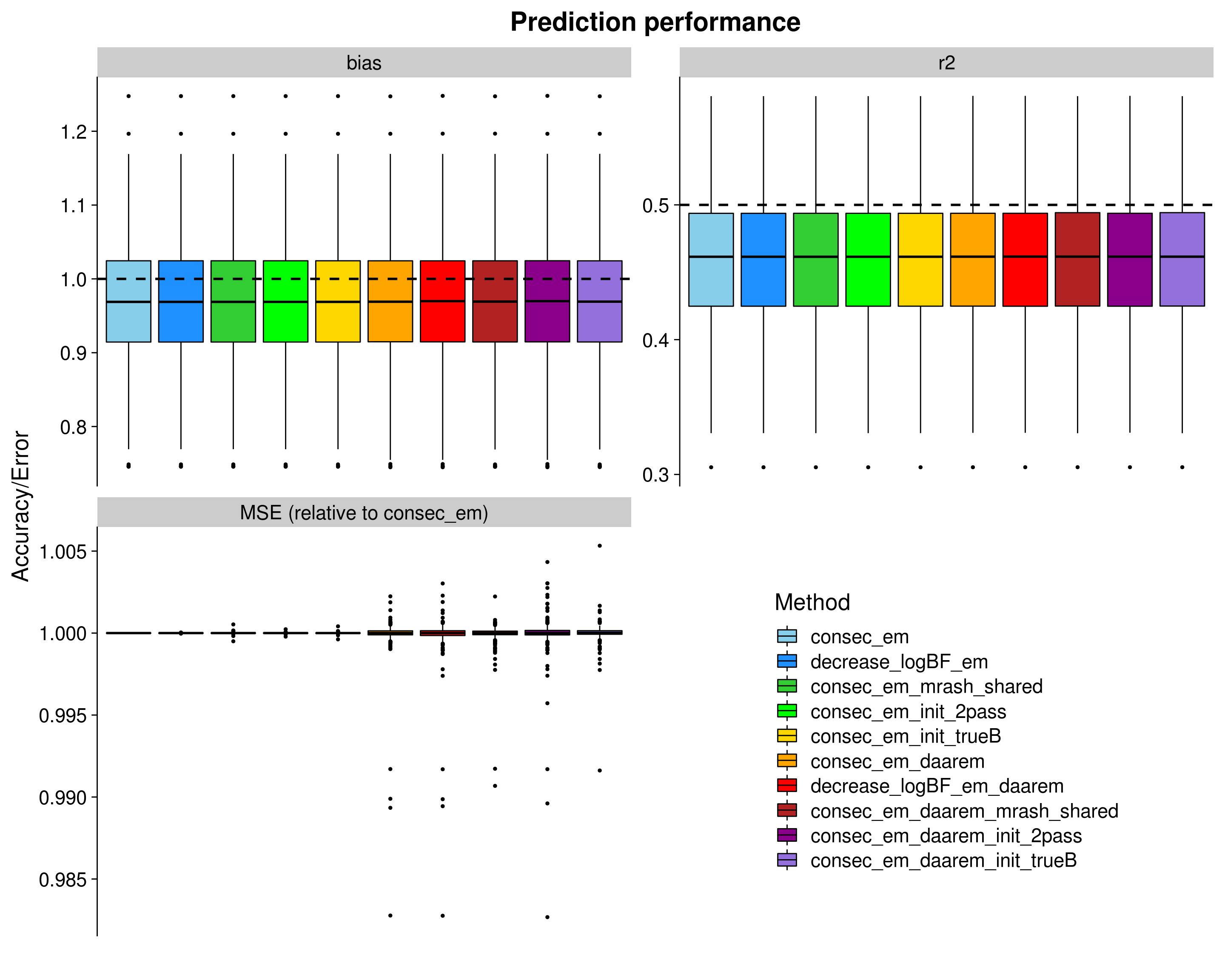
| Version | Author | Date |
|---|---|---|
| 4263395 | fmorgante | 2020-05-20 |
Let’s now remove outliers from the rMSE plot to make things a little clearer.
p_rmse_nooutliers <- ggplot(dsc_plots[which(dsc_plots$score_metric=="rmse"), ], aes_string(x = "method_fac", y = "score_value", fill = "method_fac")) +
  Ipaper::geom_boxplot2(color = "black", outlier.size = 1, width = 0.85, width.errorbar = 0) +
  scale_fill_manual(values = colors) +
  labs(x = "", y = "Relative error", title = "rMSE (relative to consec_em)", fill="Method") +
  theme_cowplot(font_size = 20) +
  theme(axis.line.x = element_blank(), axis.text.x = element_blank(), axis.ticks.x = element_blank(),
        plot.title = element_text(hjust = 0.5))

print(p_rmse_nooutliers)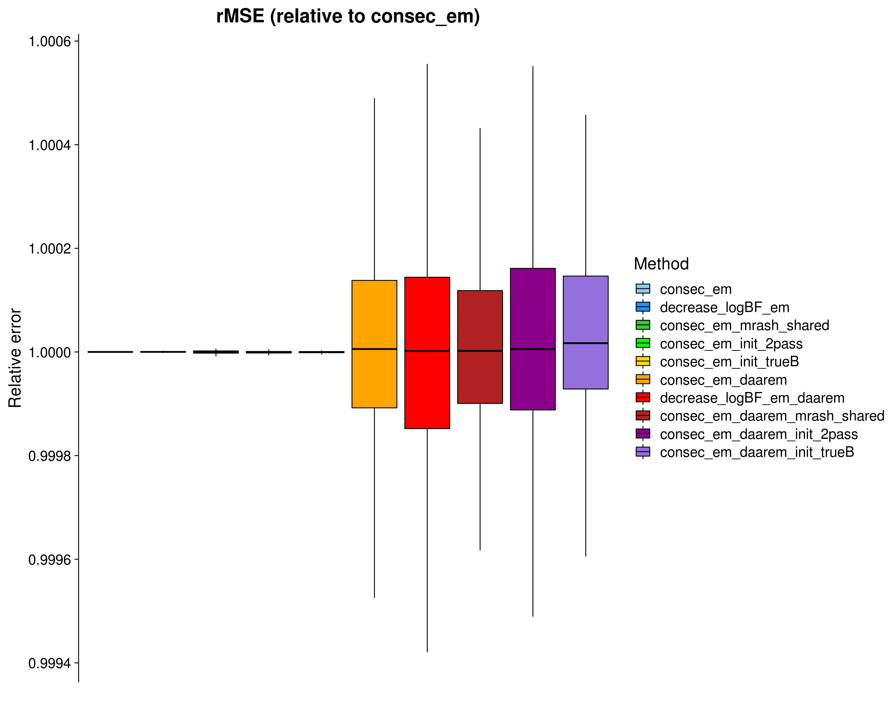
| Version | Author | Date |
|---|---|---|
| 4263395 | fmorgante | 2020-05-20 |
Here, we look at the elapsed time (\(log_{10}\) seconds) of mr.mash. Note that this time does not include the run time of mr.ash in the cases where we used it to initialize the posterior means of the regression coefficients.
dsc_plots_time <- dsc_plots[which(dsc_plots$response==1 & dsc_plots$score_metric=="r2"),
                          -which(colnames(dsc_plots) %in% c("score_metric", "score_value", "response"))]

p_time <- ggplot(dsc_plots_time, aes_string(x = "method_fac", y = "time", fill = "method_fac")) +
  geom_boxplot(color = "black", outlier.size = 1, width = 0.85) +
  scale_fill_manual(values = colors) +
  scale_y_continuous(trans="log10", breaks = trans_breaks("log10", function(x) 10^x),
                      labels = trans_format("log10", math_format(10^.x))) +
  labs(x = "", y = "Elapsed time (seconds) in log10 scale",title = "Run time", fill="Method") +
  theme_cowplot(font_size = 20) +
  theme(axis.line.x = element_blank(), axis.text.x = element_blank(), axis.ticks.x = element_blank(),
        plot.title = element_text(hjust = 0.5))

print(p_time)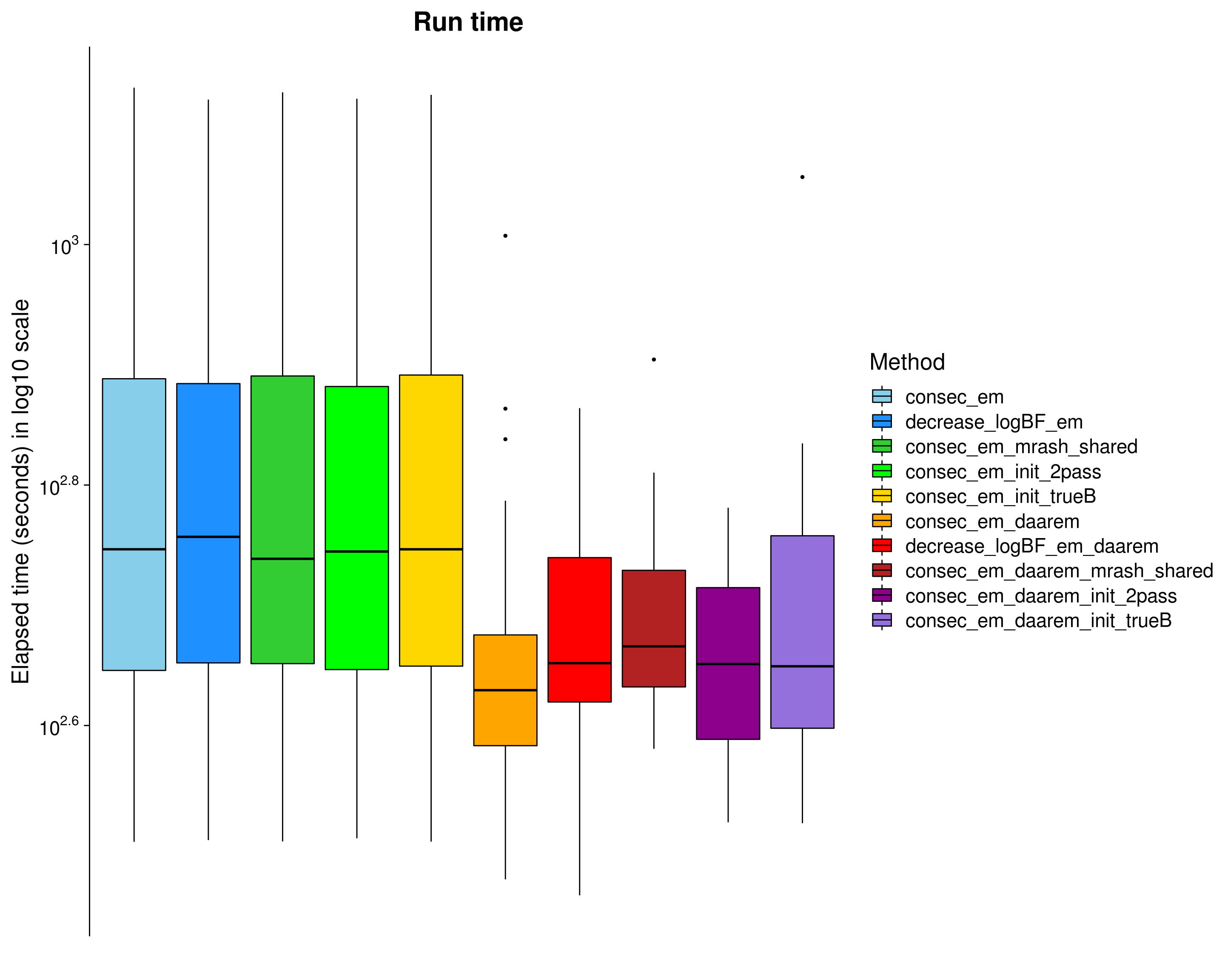
| Version | Author | Date |
|---|---|---|
| 4263395 | fmorgante | 2020-05-20 |
mr.mash vs other methods
Here, we compare mr.mash to the multivariate versions of LASSO, Elastic Net (\(\alpha = 0.5\)), and Ridge Regression as implemented in glmnet. The form of the penalty id the following: \(\lambda[(1-\alpha)/2 ||\mathbf{\beta}_j||^2_2 + \alpha ||\mathbf{\beta}_j||_2]\). \(\lambda\) is chosen by cross-validation in the training set.
###Convert from list to data.frame for plotting
dsc_plots <- convert_dsc_to_dataframe(dsc_out)

###Compute rmse score (relative to mr_mash_consec_em) and add it to the data
rmse_dat <- compute_rmse(dsc_plots)
dsc_plots <- rbind(dsc_plots, rmse_dat)

###Remove mse from scores and keep only methods wanted
dsc_plots <- dsc_plots[which(dsc_plots$score_metric!="mse" & dsc_plots$method %in% c("mr_mash_consec_em", "mr_mash_consec_em_init_mlasso",
                                                          "mr_mash_consec_em_init_trueB", "mlasso", "menet", "mridge")), ]

###Create factor version of method
dsc_plots$method_fac <- factor(dsc_plots$method, levels=c("mr_mash_consec_em", "mr_mash_consec_em_init_mlasso",
                                                          "mr_mash_consec_em_init_trueB", "mlasso", "menet", "mridge"),
                                                labels=c("consec_em", "consec_em_init_mlasso", "consec_em_init_trueB",
                                                         "mlasso", "menet", "mridge"))

###Build data.frame with best accuracy achievable
hlines <- data.frame(score_metric=c("r2", "bias"), max_val=c(unique(dsc_plots$pve), 1))

###Create plots
p <- ggplot(dsc_plots, aes_string(x = "method_fac", y = "score_value", fill = "method_fac")) +
    geom_boxplot(color = "black", outlier.size = 1, width = 0.85) +
    facet_wrap(vars(score_metric), scales="free_y", ncol=2, labeller=labeller(score_metric=facet_labels)) +
    scale_fill_manual(values = colors) +
    labs(x = "", y = "Accuracy/Error", title = "Prediction performance", fill="Method") +
    geom_hline(data=hlines, aes(yintercept = max_val), linetype="dashed", size=1) +
    theme_cowplot(font_size = 20) +
    theme(axis.line.x = element_blank(), axis.text.x = element_blank(), axis.ticks.x = element_blank(),
          plot.title = element_text(hjust = 0.5))

shift_legend(p)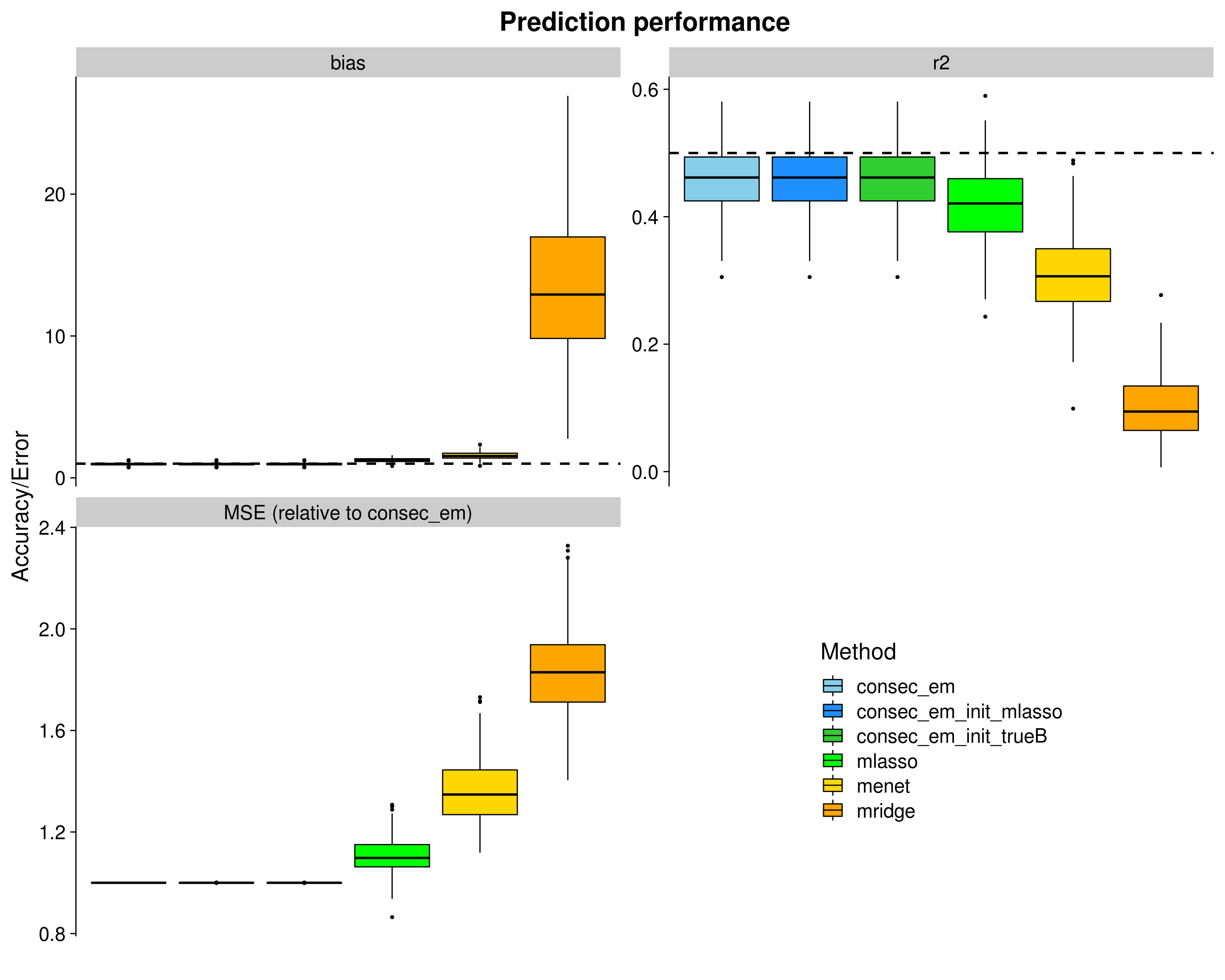
| Version | Author | Date |
|---|---|---|
| 9f85985 | fmorgante | 2020-05-25 |
Let’s now remove outliers from the rMSE plot to make things a little clearer.
p_rmse_nooutliers <- ggplot(dsc_plots[which(dsc_plots$score_metric=="rmse"), ], aes_string(x = "method_fac", y = "score_value", fill = "method_fac")) +
  Ipaper::geom_boxplot2(color = "black", outlier.size = 1, width = 0.85, width.errorbar = 0) +
  scale_fill_manual(values = colors) +
  labs(x = "", y = "Relative error", title = "rMSE (relative to consec_em)", fill="Method") +
  theme_cowplot(font_size = 20) +
  theme(axis.line.x = element_blank(), axis.text.x = element_blank(), axis.ticks.x = element_blank(),
        plot.title = element_text(hjust = 0.5))

print(p_rmse_nooutliers)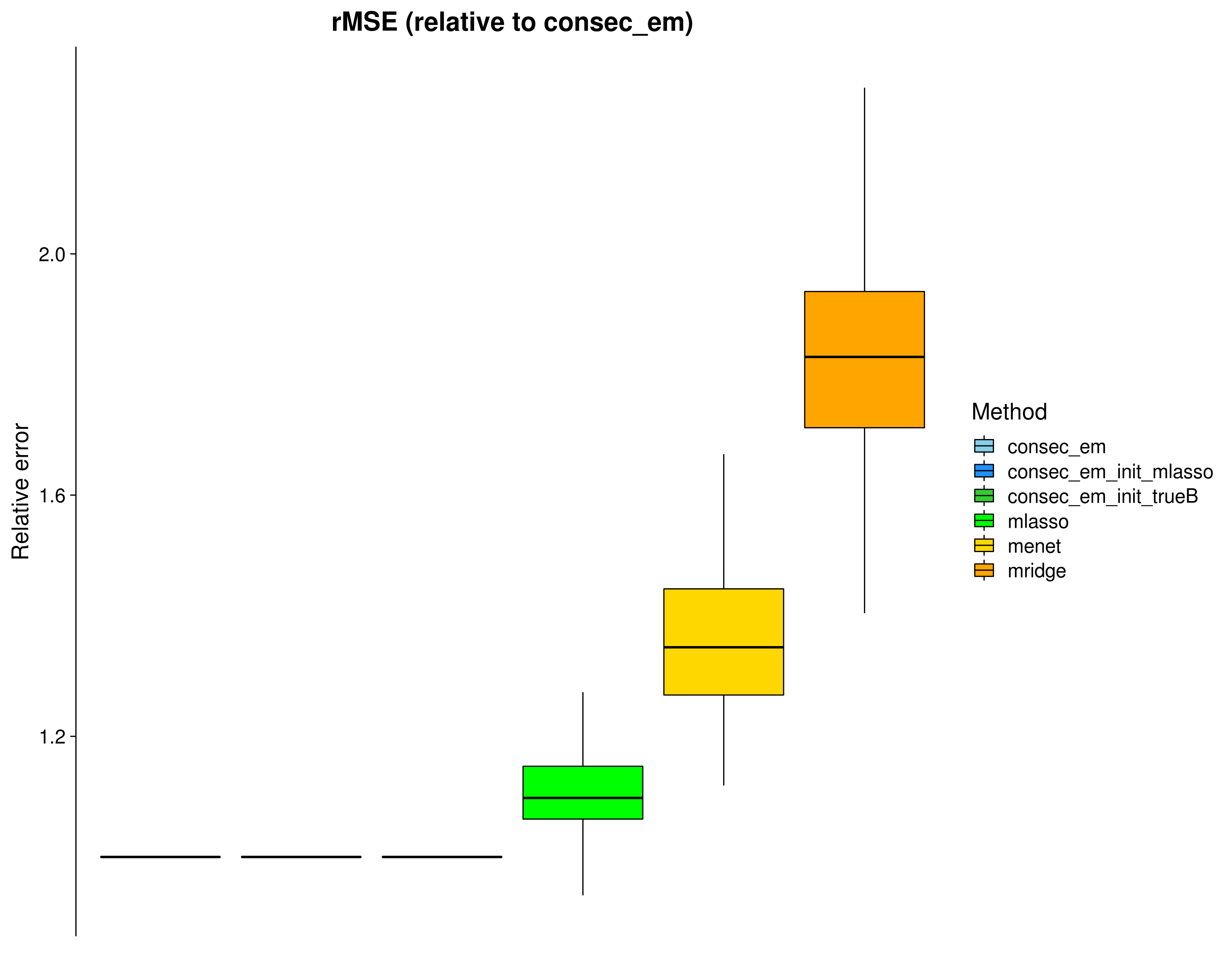
| Version | Author | Date |
|---|---|---|
| 9f85985 | fmorgante | 2020-05-25 |
Here, we look at the elapsed time (\(log_{10}\) seconds) of mr.mash. Note that this time does not include the run time of glmnet in the cases where we used it to initialize the posterior means of the regression coefficients.
dsc_plots_time <- dsc_plots[which(dsc_plots$response==1 & dsc_plots$score_metric=="r2"),
                          -which(colnames(dsc_plots) %in% c("score_metric", "score_value", "response"))]

p_time <- ggplot(dsc_plots_time, aes_string(x = "method_fac", y = "time", fill = "method_fac")) +
  geom_boxplot(color = "black", outlier.size = 1, width = 0.85) +
  scale_fill_manual(values = colors) +
  scale_y_continuous(trans="log10", breaks = trans_breaks("log10", function(x) 10^x),
                      labels = trans_format("log10", math_format(10^.x))) +
  labs(x = "", y = "Elapsed time (seconds) in log10 scale",title = "Run time", fill="Method") +
  theme_cowplot(font_size = 20) +
  theme(axis.line.x = element_blank(), axis.text.x = element_blank(), axis.ticks.x = element_blank(),
        plot.title = element_text(hjust = 0.5))

print(p_time)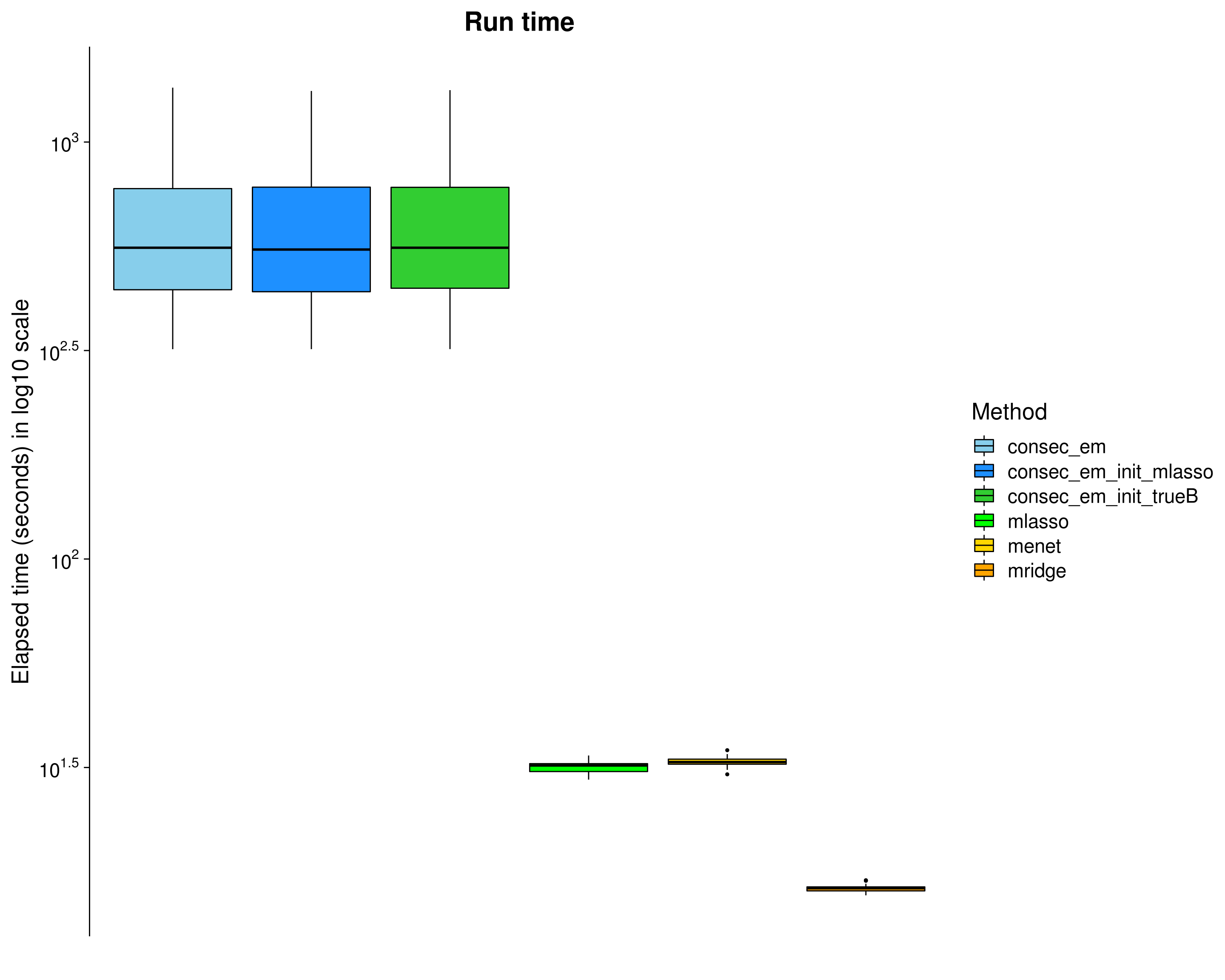
| Version | Author | Date |
|---|---|---|
| 9f85985 | fmorgante | 2020-05-25 |
###Load the dsc results
dsc_out <- dscquery("output/dsc_05_18_20", c("simulate.n", "simulate.p", "simulate.p_causal", "simulate.r",
                                 "simulate.pve", "simulate.B_cor", "simulate.B_scale",
                                 "simulate.X_cor", "simulate.X_scale",
                                 "simulate.V_cor", "simulate.prop_testset",
                                 "simulate", "fit", "score", "score.err", "fit.time"),
                    conditions = "$(simulate) == 'indepX_lowcorrV_sharedB' & $(simulate.p_causal) == 500", verbose=FALSE,
                    ignore.missing.files = TRUE )

###Obtain simulation parameters
n <- unique(dsc_out$simulate.n)
p <- unique(dsc_out$simulate.p)
p_causal <- unique(dsc_out$simulate.p_causal)
r <- unique(dsc_out$simulate.r)
k <- 166
pve <- unique(dsc_out$simulate.pve)
prop_testset <- unique(dsc_out$simulate.prop_testset)
B_cor <- unique(dsc_out$simulate.B_cor)
B_scale <- unique(dsc_out$simulate.B_scale)
X_cor <- unique(dsc_out$simulate.X_cor)
X_scale <- unique(dsc_out$simulate.X_scale)
V_cor <- unique(dsc_out$simulate.V_cor)

###Remove list elements that are not useful anymore
dsc_out$simulate.prop_testset <- NULL
dsc_out$simulate.B_cor <- NULL
dsc_out$simulate.B_scale <- NULL
dsc_out$simulate.X_cor <- NULL
dsc_out$simulate.X_scale <- NULL
dsc_out$simulate.V_cor <- NULL
500 causal variables
The results below are based on the same simulation/analysis scheme as above but with 500 causal variables.
###Convert from list to data.frame for plotting
dsc_plots <- convert_dsc_to_dataframe(dsc_out)

###Compute rmse score (relative to mr_mash_consec_em) and add it to the data
rmse_dat <- compute_rmse(dsc_plots)
dsc_plots <- rbind(dsc_plots, rmse_dat)

###Remove mse from scores and keep only methods wanted
dsc_plots <- dsc_plots[which(dsc_plots$score_metric!="mse" & dsc_plots$method %in% c("mr_mash_consec_em", "mr_mash_declogBF_em",
                                                          "mr_mash_consec_em_init_shared", "mr_mash_consec_em_init_2pass",
                                                          "mr_mash_consec_em_init_trueB",
                                                          "mr_mash_consec_em_daarem", "mr_mash_declogBF_em_daarem",
                                                          "mr_mash_consec_em_daarem_init_shared", "mr_mash_consec_em_daarem_init_2pass",
                                                          "mr_mash_consec_em_daarem_init_trueB")), ]

###Create factor version of method
dsc_plots$method_fac <- factor(dsc_plots$method, levels=c("mr_mash_consec_em", "mr_mash_declogBF_em",
                                                          "mr_mash_consec_em_init_shared", "mr_mash_consec_em_init_2pass",
                                                          "mr_mash_consec_em_init_trueB",
                                                          "mr_mash_consec_em_daarem", "mr_mash_declogBF_em_daarem",
                                                          "mr_mash_consec_em_daarem_init_shared", "mr_mash_consec_em_daarem_init_2pass",
                                                          "mr_mash_consec_em_daarem_init_trueB"),
                                                labels=c("consec_em", "decrease_logBF_em", "consec_em_mrash_shared",
                                                         "consec_em_init_2pass", "consec_em_init_trueB",
                                                         "consec_em_daarem", "decrease_logBF_em_daarem", "consec_em_daarem_mrash_shared",
                                                         "consec_em_daarem_init_2pass", "consec_em_daarem_init_trueB"))

###Build data.frame with best accuracy achievable
hlines <- data.frame(score_metric=c("r2", "bias"), max_val=c(unique(dsc_plots$pve), 1))

###Create plots
p <- ggplot(dsc_plots, aes_string(x = "method_fac", y = "score_value", fill = "method_fac")) +
    geom_boxplot(color = "black", outlier.size = 1, width = 0.85) +
    facet_wrap(vars(score_metric), scales="free_y", ncol=2, labeller=labeller(score_metric=facet_labels)) +
    scale_fill_manual(values = colors) +
    labs(x = "", y = "Accuracy/Error", title = "Prediction performance", fill="Method") +
    geom_hline(data=hlines, aes(yintercept = max_val), linetype="dashed", size=1) +
    theme_cowplot(font_size = 20) +
    theme(axis.line.x = element_blank(), axis.text.x = element_blank(), axis.ticks.x = element_blank(),
          plot.title = element_text(hjust = 0.5))

shift_legend(p)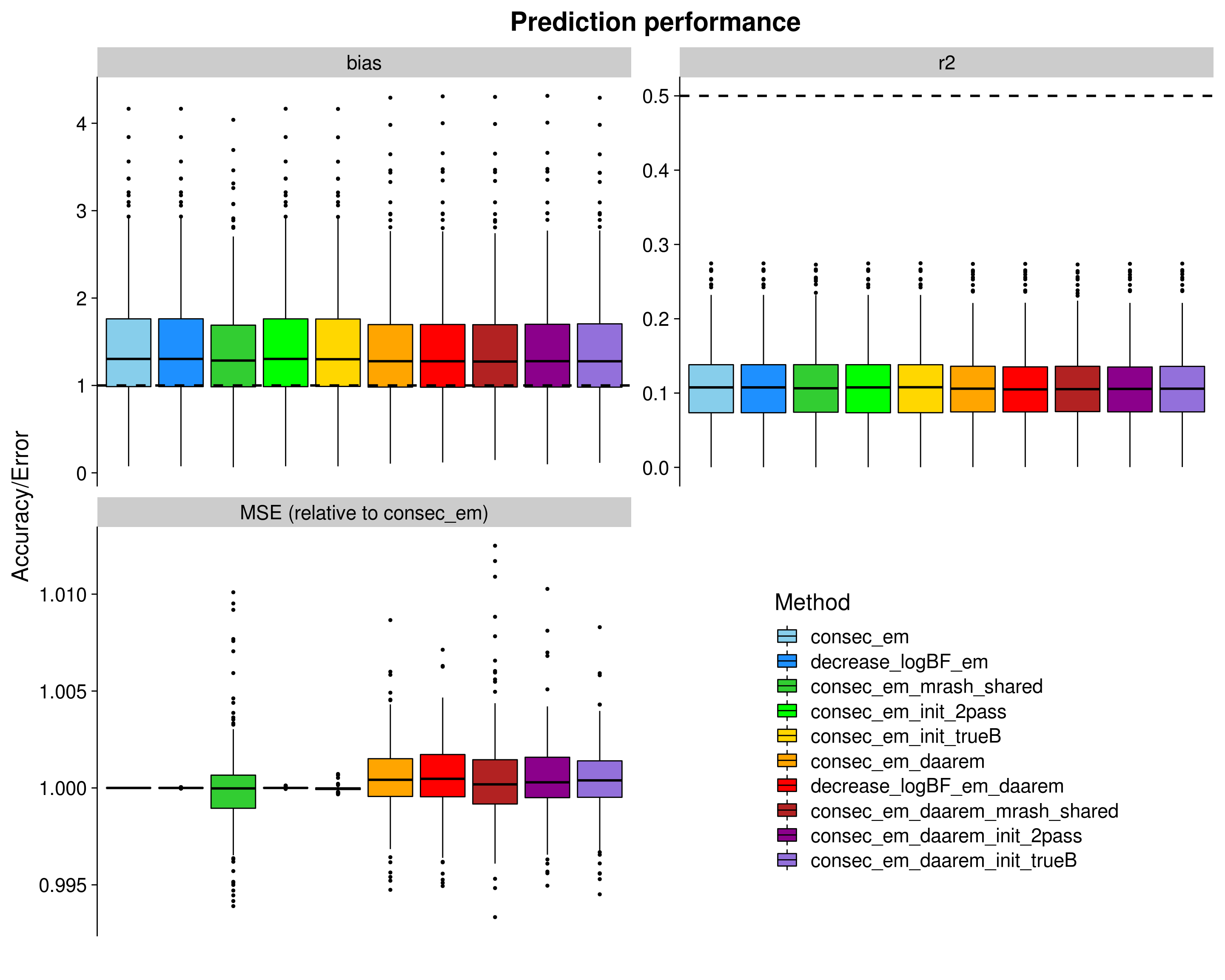
| Version | Author | Date |
|---|---|---|
| 4263395 | fmorgante | 2020-05-20 |
Let’s now remove outliers from the rMSE plot to make things a little clearer.
p_rmse_nooutliers <- ggplot(dsc_plots[which(dsc_plots$score_metric=="rmse"), ], aes_string(x = "method_fac", y = "score_value", fill = "method_fac")) +
  Ipaper::geom_boxplot2(color = "black", outlier.size = 1, width = 0.85, width.errorbar = 0) +
  scale_fill_manual(values = colors) +
  labs(x = "", y = "Relative error", title = "rMSE (relative to consec_em)", fill="Method") +
  theme_cowplot(font_size = 20) +
  theme(axis.line.x = element_blank(), axis.text.x = element_blank(), axis.ticks.x = element_blank(),
        plot.title = element_text(hjust = 0.5))

print(p_rmse_nooutliers)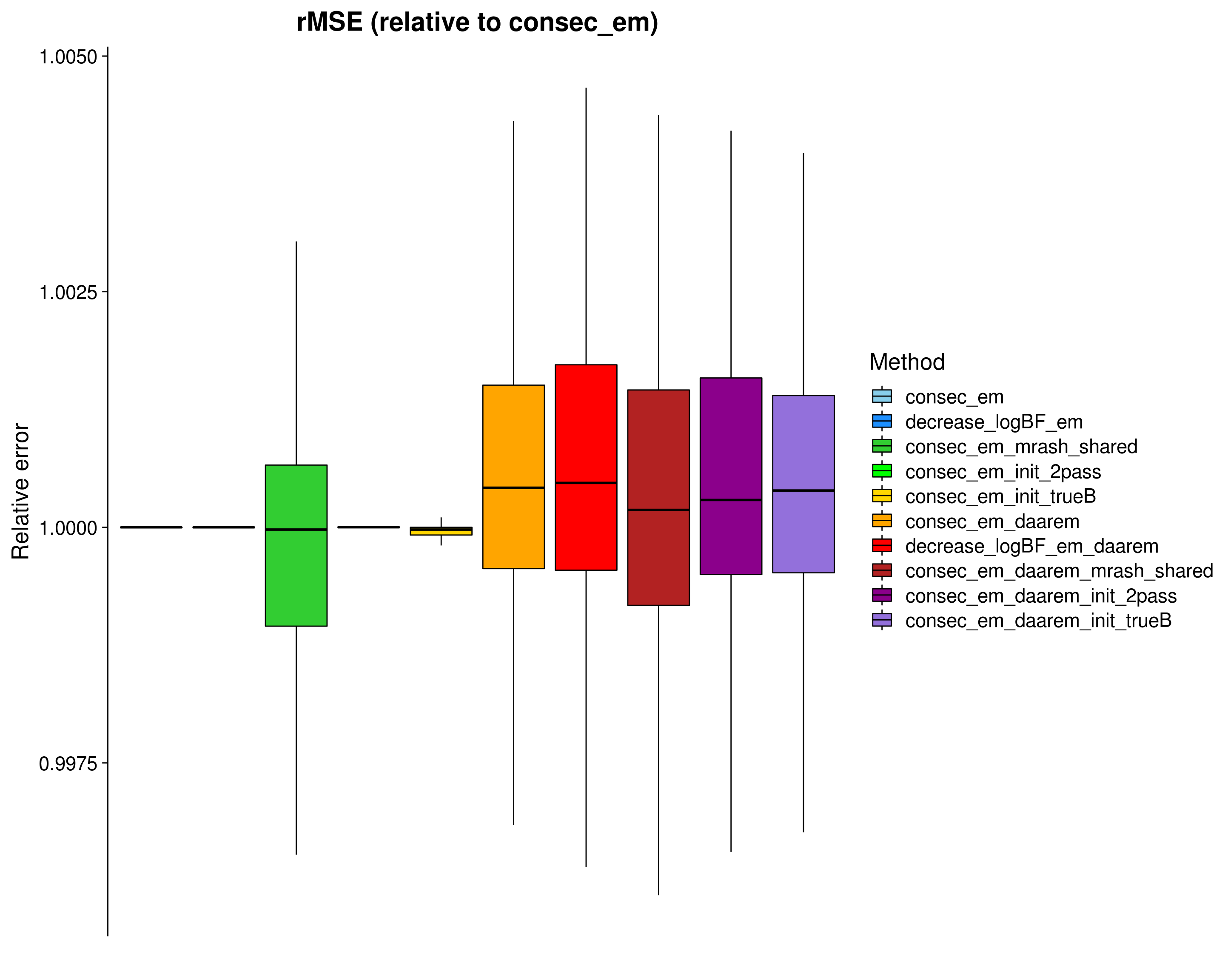
| Version | Author | Date |
|---|---|---|
| 4263395 | fmorgante | 2020-05-20 |
Here, we look at the elapsed time (\(log_{10}\) seconds) of mr.mash. Note that this time does not include the run time of mr.ash in the cases where we used it to initialize the posterior means of the regression coefficients.
dsc_plots_time <- dsc_plots[which(dsc_plots$response==1 & dsc_plots$score_metric=="r2"),
                          -which(colnames(dsc_plots) %in% c("score_metric", "score_value", "response"))]

p_time <- ggplot(dsc_plots_time, aes_string(x = "method_fac", y = "time", fill = "method_fac")) +
  geom_boxplot(color = "black", outlier.size = 1, width = 0.85) +
  scale_fill_manual(values = colors) +
  scale_y_continuous(trans="log10", breaks = trans_breaks("log10", function(x) 10^x),
                      labels = trans_format("log10", math_format(10^.x))) +
  labs(x = "", y = "Elapsed time (seconds) in log10 scale",title = "Run time", fill="Method") +
  theme_cowplot(font_size = 20) +
  theme(axis.line.x = element_blank(), axis.text.x = element_blank(), axis.ticks.x = element_blank(),
        plot.title = element_text(hjust = 0.5))

print(p_time)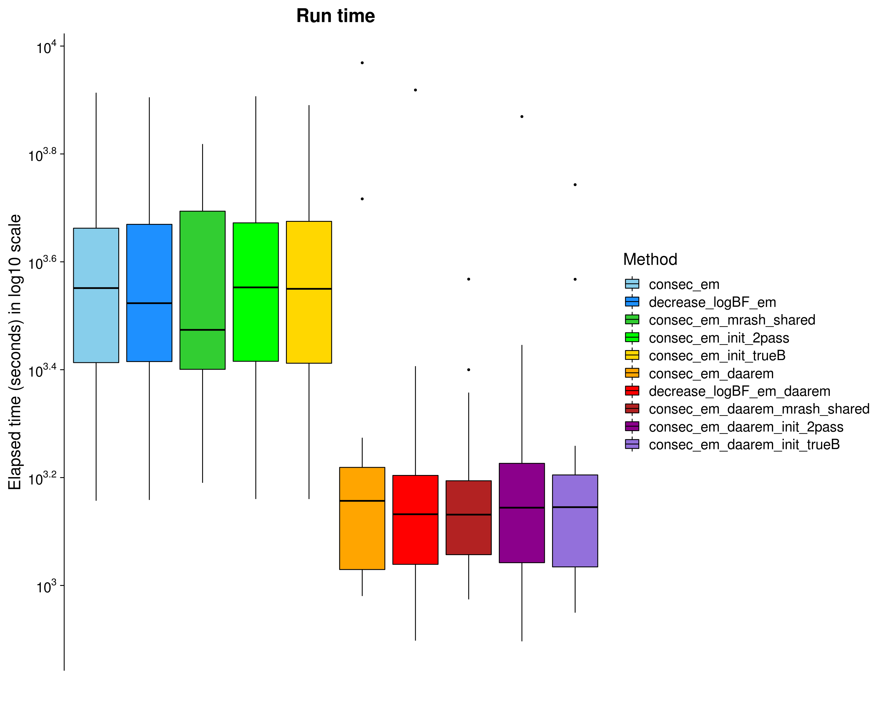
| Version | Author | Date |
|---|---|---|
| 4263395 | fmorgante | 2020-05-20 |
mr.mash vs other methods
Here, we compare mr.mash to the multivariate versions of LASSO, Elastic Net (\(\alpha = 0.5\)), and Ridge Regression as implemented in glmnet. The form of the penalty id the following: \(\lambda[(1-\alpha)/2 ||\mathbf{\beta}_j||^2_2 + \alpha ||\mathbf{\beta}_j||_2]\). \(\lambda\) is chosen by cross-validation in the training set.
###Convert from list to data.frame for plotting
dsc_plots <- convert_dsc_to_dataframe(dsc_out)

###Compute rmse score (relative to mr_mash_consec_em) and add it to the data
rmse_dat <- compute_rmse(dsc_plots)
dsc_plots <- rbind(dsc_plots, rmse_dat)

###Remove mse from scores and keep only methods wanted
dsc_plots <- dsc_plots[which(dsc_plots$score_metric!="mse" & dsc_plots$method %in% c("mr_mash_consec_em", "mr_mash_consec_em_init_mlasso",
                                                          "mr_mash_consec_em_init_trueB", "mlasso", "menet", "mridge")), ]

###Create factor version of method
dsc_plots$method_fac <- factor(dsc_plots$method, levels=c("mr_mash_consec_em", "mr_mash_consec_em_init_mlasso",
                                                          "mr_mash_consec_em_init_trueB", "mlasso", "menet", "mridge"),
                                                labels=c("consec_em", "consec_em_init_mlasso", "consec_em_init_trueB",
                                                         "mlasso", "menet", "mridge"))

###Build data.frame with best accuracy achievable
hlines <- data.frame(score_metric=c("r2", "bias"), max_val=c(unique(dsc_plots$pve), 1))

###Create plots
p <- ggplot(dsc_plots, aes_string(x = "method_fac", y = "score_value", fill = "method_fac")) +
    geom_boxplot(color = "black", outlier.size = 1, width = 0.85) +
    facet_wrap(vars(score_metric), scales="free_y", ncol=2, labeller=labeller(score_metric=facet_labels)) +
    scale_fill_manual(values = colors) +
    labs(x = "", y = "Accuracy/Error", title = "Prediction performance", fill="Method") +
    geom_hline(data=hlines, aes(yintercept = max_val), linetype="dashed", size=1) +
    theme_cowplot(font_size = 20) +
    theme(axis.line.x = element_blank(), axis.text.x = element_blank(), axis.ticks.x = element_blank(),
          plot.title = element_text(hjust = 0.5))

shift_legend(p)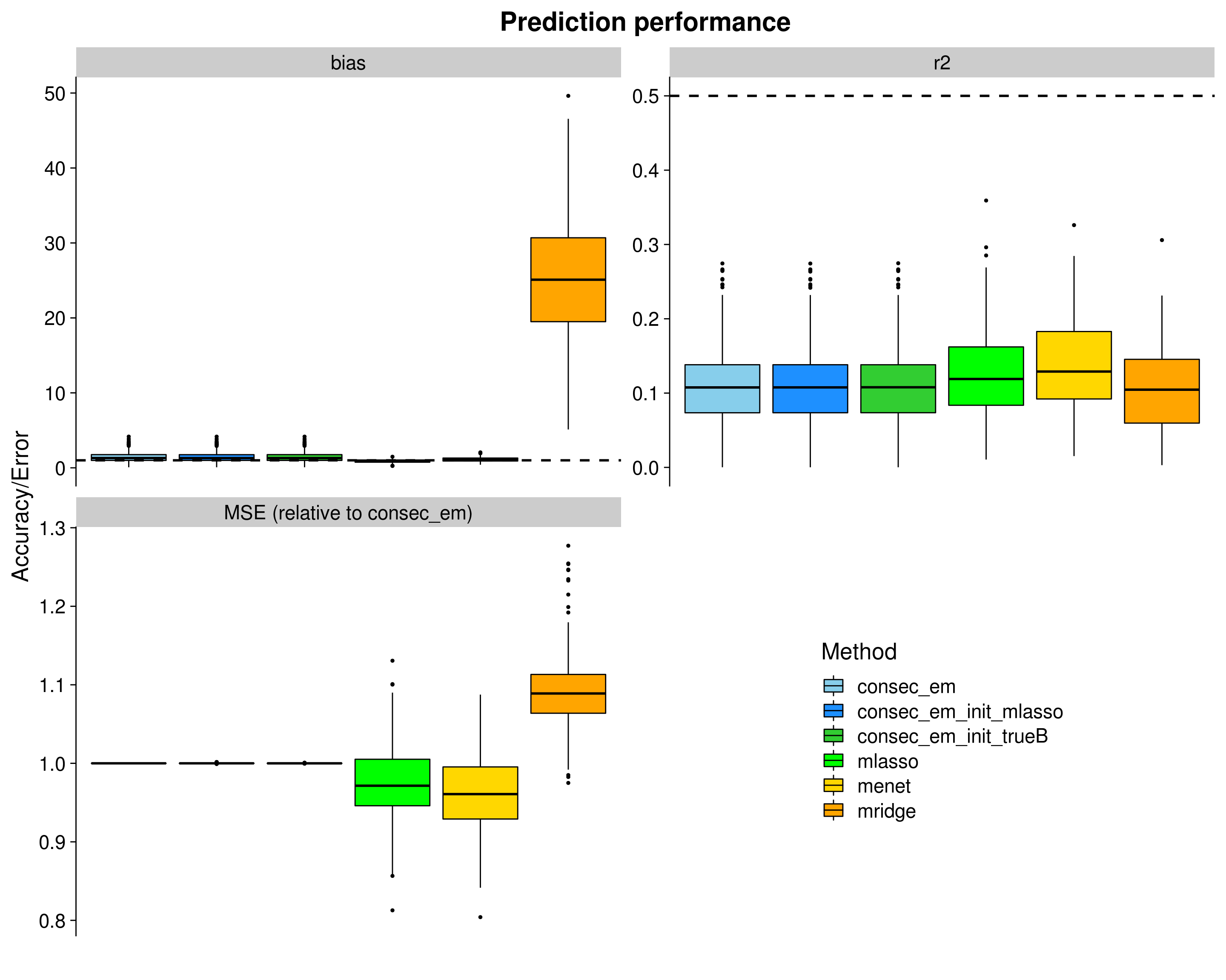
| Version | Author | Date |
|---|---|---|
| 9f85985 | fmorgante | 2020-05-25 |
Let’s now remove outliers from the rMSE plot to make things a little clearer.
p_rmse_nooutliers <- ggplot(dsc_plots[which(dsc_plots$score_metric=="rmse"), ], aes_string(x = "method_fac", y = "score_value", fill = "method_fac")) +
  Ipaper::geom_boxplot2(color = "black", outlier.size = 1, width = 0.85, width.errorbar = 0) +
  scale_fill_manual(values = colors) +
  labs(x = "", y = "Relative error", title = "rMSE (relative to consec_em)", fill="Method") +
  theme_cowplot(font_size = 20) +
  theme(axis.line.x = element_blank(), axis.text.x = element_blank(), axis.ticks.x = element_blank(),
        plot.title = element_text(hjust = 0.5))

print(p_rmse_nooutliers)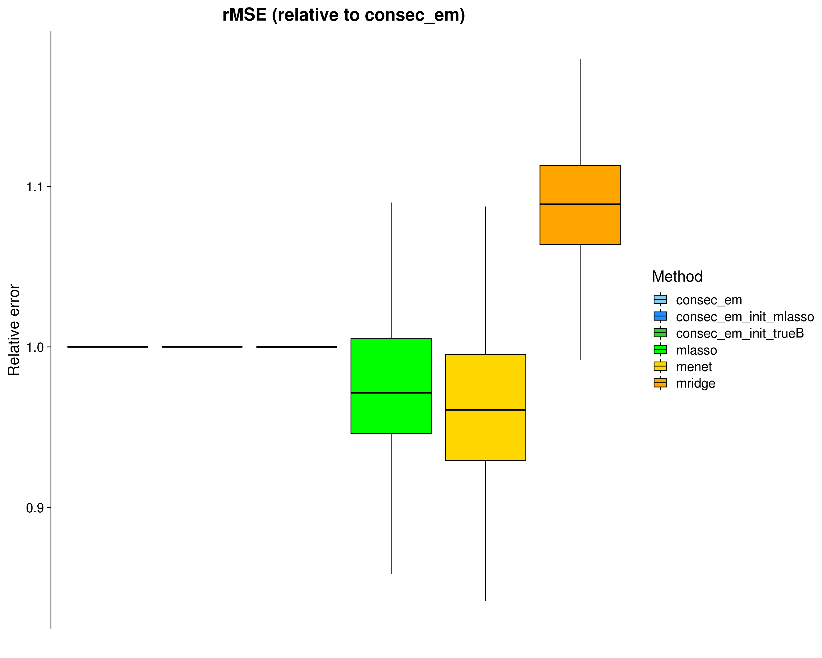
| Version | Author | Date |
|---|---|---|
| 9f85985 | fmorgante | 2020-05-25 |
Here, we look at the elapsed time (\(log_{10}\) seconds) of mr.mash. Note that this time does not include the run time of glmnet in the cases where we used it to initialize the posterior means of the regression coefficients.
dsc_plots_time <- dsc_plots[which(dsc_plots$response==1 & dsc_plots$score_metric=="r2"),
                          -which(colnames(dsc_plots) %in% c("score_metric", "score_value", "response"))]

p_time <- ggplot(dsc_plots_time, aes_string(x = "method_fac", y = "time", fill = "method_fac")) +
  geom_boxplot(color = "black", outlier.size = 1, width = 0.85) +
  scale_fill_manual(values = colors) +
  scale_y_continuous(trans="log10", breaks = trans_breaks("log10", function(x) 10^x),
                      labels = trans_format("log10", math_format(10^.x))) +
  labs(x = "", y = "Elapsed time (seconds) in log10 scale",title = "Run time", fill="Method") +
  theme_cowplot(font_size = 20) +
  theme(axis.line.x = element_blank(), axis.text.x = element_blank(), axis.ticks.x = element_blank(),
        plot.title = element_text(hjust = 0.5))

print(p_time)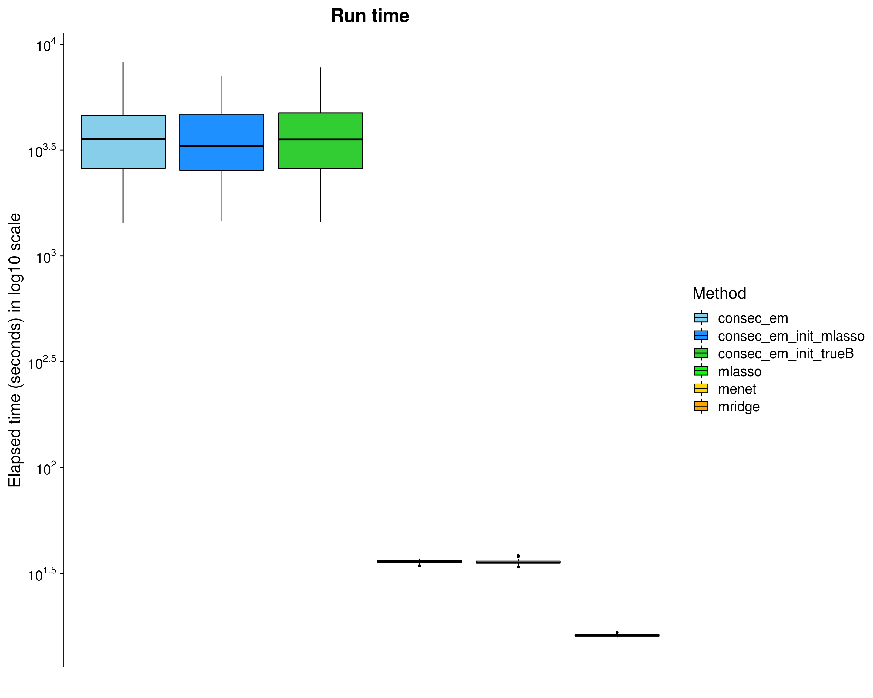
| Version | Author | Date |
|---|---|---|
| 9f85985 | fmorgante | 2020-05-25 |
sessionInfo()R version 3.5.1 (2018-07-02)
Platform: x86_64-pc-linux-gnu (64-bit)
Running under: Scientific Linux 7.4 (Nitrogen)
Matrix products: default
BLAS/LAPACK: /software/openblas-0.2.19-el7-x86_64/lib/libopenblas_haswellp-r0.2.19.so
locale:
[1] LC_CTYPE=en_US.UTF-8 LC_NUMERIC=C
[3] LC_TIME=en_US.UTF-8 LC_COLLATE=en_US.UTF-8
[5] LC_MONETARY=en_US.UTF-8 LC_MESSAGES=en_US.UTF-8
[7] LC_PAPER=en_US.UTF-8 LC_NAME=C
[9] LC_ADDRESS=C LC_TELEPHONE=C
[11] LC_MEASUREMENT=en_US.UTF-8 LC_IDENTIFICATION=C
attached base packages:
[1] stats graphics grDevices utils datasets methods base
other attached packages:
[1] devtools_2.1.0 usethis_1.5.1 magrittr_1.5 lemon_0.4.3
[5] gtable_0.3.0 scales_1.1.0 cowplot_1.0.0 ggplot2_3.2.0
[9] dscrutils_0.4.2
loaded via a namespace (and not attached):
[1] pkgload_1.0.2 jsonlite_1.6 foreach_1.4.4
[4] Ipaper_0.1.5 assertthat_0.2.1 sp_1.3-1
[7] cellranger_1.1.0 yaml_2.2.1 remotes_2.1.0
[10] progress_1.2.2 sessioninfo_1.1.1 pillar_1.4.1
[13] backports_1.1.5 lattice_0.20-38 glue_1.4.0
[16] digest_0.6.25 RColorBrewer_1.1-2 promises_1.0.1
[19] colorspace_1.4-1 htmltools_0.3.6 httpuv_1.4.5
[22] plyr_1.8.5 clipr_0.4.1 pkgconfig_2.0.3
[25] purrr_0.3.3 processx_3.4.0 whisker_0.3-2
[28] openxlsx_4.1.0 later_0.7.5 git2r_0.26.1
[31] tibble_2.1.3 farver_2.0.3 withr_2.1.2
[34] repr_0.17 lazyeval_0.2.2 cli_1.1.0
[37] crayon_1.3.4 readxl_1.1.0 memoise_1.1.0
[40] evaluate_0.12 ps_1.2.1 fs_1.3.1
[43] doParallel_1.0.14 xml2_1.2.0 pkgbuild_1.0.3
[46] tools_3.5.1 data.table_1.12.8 prettyunits_1.1.1
[49] hms_0.5.3 matrixStats_0.55.0 lifecycle_0.2.0
[52] stringr_1.4.0 munsell_0.5.0 zip_1.0.0
[55] callr_3.3.2 compiler_3.5.1 rlang_0.4.5
[58] grid_3.5.1 rstudioapi_0.10 iterators_1.0.10
[61] base64enc_0.1-3 labeling_0.3 rmarkdown_1.10
[64] boot_1.3-20 testthat_2.1.1 codetools_0.2-15
[67] reshape2_1.4.3 R6_2.4.1 lubridate_1.7.4
[70] gridExtra_2.3 knitr_1.20 dplyr_0.8.0.1
[73] workflowr_1.6.1 rprojroot_1.3-2 desc_1.2.0
[76] stringi_1.4.3 parallel_3.5.1 IRdisplay_0.6.1
[79] Rcpp_1.0.4.6 vctrs_0.2.4 tidyselect_0.2.5